Plot

Plot module have three submodules.

FW (Feature weights)
cor (Feature Correlation (cor) analysis)
IFS (Incremental feature selection curves)
SHAP (shap values summary)
waterfall (Feature waterfall based on shap values)
beeswarm (Feature beeswarm based on shap values of specific category)
PCA (Principal component analysis)
CM (Confusion matrix)

Feature Weights (FW)

FW module shows the feature selection method to plot the contribution of each feature.

Parameters	Optional	Descripton
-i, —input	filename path	Feature importance dataframe path (CSV format)
—format	png, pdf	Picture format
-n, —number	int (default=50)	Number of features shown in the picture
-o, —output	directory	output directory (default:Current directory)

FW example

# If you do not have a dataframe of feature importances,
# Please run $Feature_scML fs -i example.csv -m fscore
$Feature_scML plot FW -i example_fscore.csv
# get example_fscore_FeatureWeight.png in the current directory.

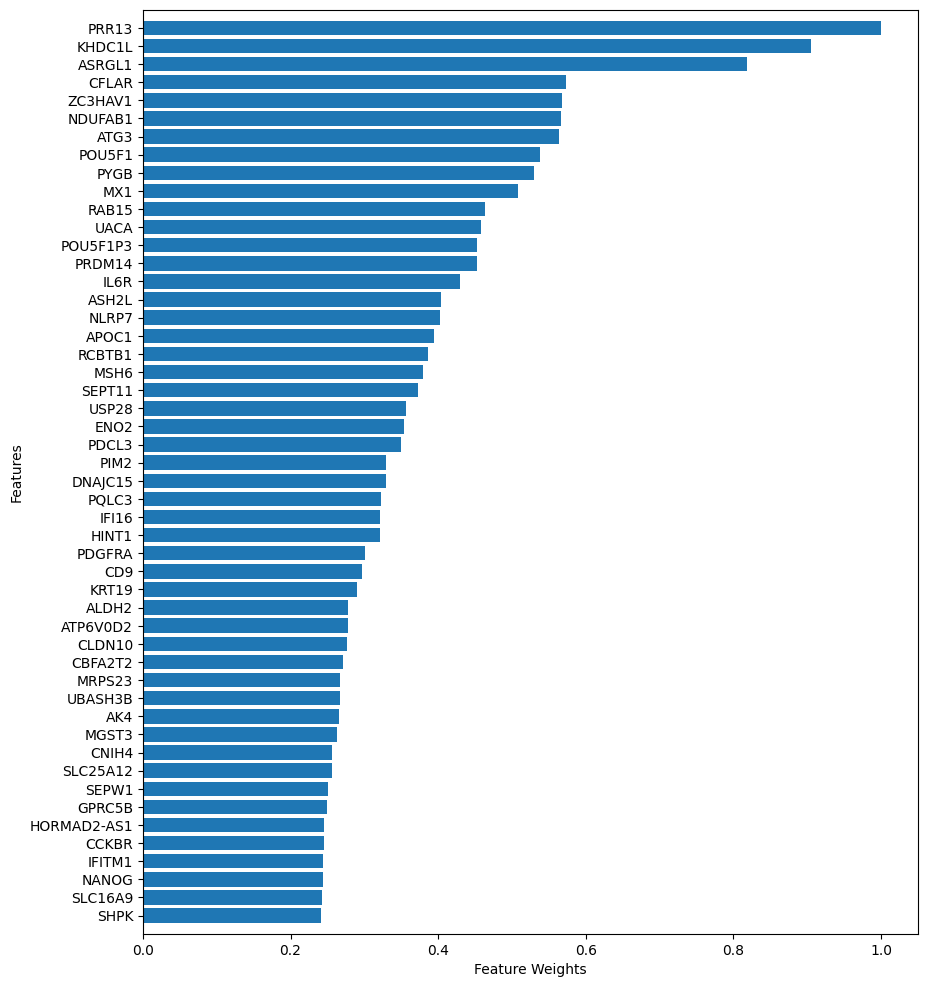
../_images/example_fscore_FeatureWeight.png — example_fscore_FeatureWeight.png

Feature Correlation (cor) analysis

cor module shows the feature correlation based on pearson, spearman, or kendall method to plot the correlation of every two features.

Parameters	Optional	Descripton
-i, —input	filename path	Feature dataframe path (CSV format)
-m, —method	pearson,spearman,kendall	correlation measure
—format	png, pdf	Picture format (default=png)
-n, —feature_number	int (default=10)	Number of top-ranked features shown in the picture
-o, —output	directory	output directory (default:Current directory)

cor example

# If you do not have a dataframe of feature importances,
# Please run $Feature_scML fs -i example.csv -m fscore
$Feature_scML plot cor -i example_fscore_data.csv -m pearson -n 10
# get pearson_correlation_example_fscore_data_10.png in the current directory.

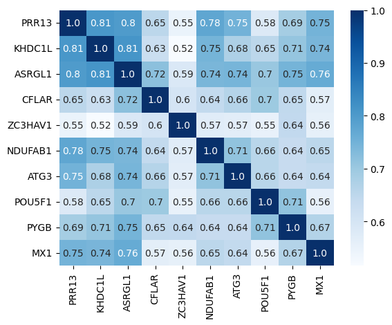
../_images/pearson_correlation_example_fscore_data_10.png — pearson_correlation_example_fscore_data_10.png

Incremental Feature Selection (IFS) Curves

IFS (incremental feature selection curves) evaluates the classification performance of the top-k-ranked features iteratively for k ∈ (1, 2, …, n), where n is the total number of features.

Parameters	Optional	Descripton
-i, —input	filename path	IFS dataframe path (CSV format)
—format	png, pdf	Picture format
-o, —output	directory	output directory (default:Current directory)

IFS example

# If you do not have a dataframe of incremental feature classification performance,
# Please run $Feature_scML automl -i example.csv -c svm -m fscore --njobs 20
$Feature_scML plot IFS -i 10-100_fscore_SVM_accuracy.csv
# get 10-100_fscore_SVM_accuracy_IFS.png in the current directory.

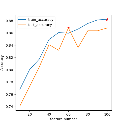
../_images/10-100_fscore_SVM_accuracy_IFS.png — 10-100_fscore_SVM_accuracy_IFS.png

SHAP

SHAP shows each feature of shap values for all categories.

Parameters	Optional	Descripton
-i, —input	filename path	dataframe path (CSV format)
—format	png, pdf	Picture format
—model_path	filename path	Model file path (joblib)
–classifier	svm,rf,lr	classifier name
-n, —feature_number	int	Consistent with the number of features trained by the model
-o, —output	directory	Output directory (default:Current directory)

SHAP example

# If you do not have a dataframe of incremental feature classification performance,
# Please run $Feature_scML automl -i example.csv -c rf -m fscore --njobs 20
$Feature_scML plot SHAP -i example.csv -c rf -n 100 --model_path example_rf.joblib

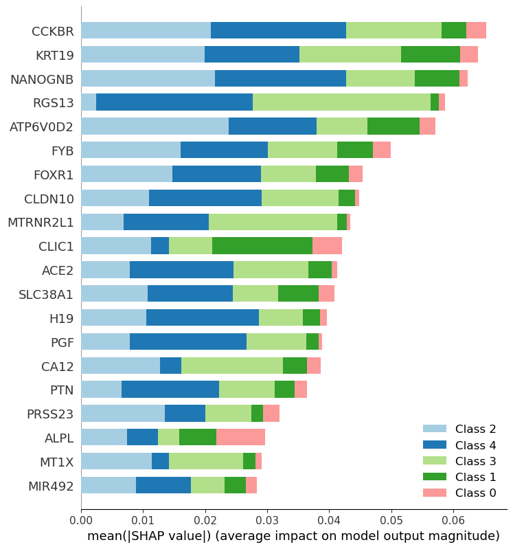
../_images/example_rf_100_SHAP_feature_summary.png — example_rf_100_SHAP_feature_summary.png

waterfall

waterfall (Feature waterfall based on shap values) shows each feature of shap values for a specific sample.

Parameters	Optional	Descripton
-i, —input	filename path	dataframe path (CSV format)
—format	png, pdf	Picture format
—model_path	filename path	Model file path (joblib)
—method	svm	Model name
-n, —feature_number	int	Consistent with the number of features trained by the model
-o, —output	directory	Output directory (default:Current directory)

waterfall example

# Feature_scML automl -i example.csv -c svm -m fscore --njobs 20 --getmodel True
$Feature_scML plot waterfall -i example_fscore_data.csv --model_path example_20_svm.joblib -s 0 -n 20

../_images/example_fscore_data_simple_feature_contribute.png — example_fscore_data_simple_feature_contribute.png

beeswarm

The beeswarm plot shows an information-dense summary of how the top features in a dataset impact the model’s output.

Parameters	Optional	Descripton
-i, —input	filename path	dataframe path (CSV format)
—format	png, pdf	Picture format
—model_path	filename path	Model file path (joblib)
—method	svm	Model name
-n, —feature_number	int	Consistent with the number of features trained by the model
-s, —sample_label	int	label category to(0, 1, …)
-o, —output	directory	Output directory (default:Current directory)

beeswarm example

# Feature_scML automl -i example.csv -c svm -m fscore --njobs 20 --getmodel True
# Evaluate the summary shap value of all samples with a strategy of 1.
$Feature_scML plot beeswarm -i example_fscore_data.csv --model_path example_20_svm.joblib  -n 20 -s 1

../_images/example_fscore_data_simple_feature_summary.png — example_fscore_data_simple_feature_summary.png

Principal Component Analysis (PCA)

The PCA plot shows the influence of different feature clustering on sample clustering.

Parameters	Optional	Descripton
-i, —input	filename path	dataframe path (CSV format)
—format	png, pdf	Picture format
-n, —feature_number	int	feature number
-o, —output	directory	Output directory (default:Current directory)

PCA example

$Feature_scML plot PCA -i example_fscore_data.csv -n 100

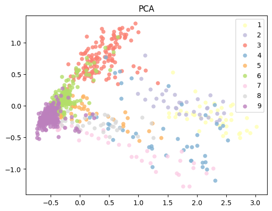
../_images/example_fscore_data_100_PCA.png — example_fscore_data_100_PCA.png

T-distributed Stochastic Neighbor Embedding (T-SNE)

The T-SNE plot shows the influence of different feature clustering on sample clustering.

Parameters	Optional	Descripton
-i, —input	filename path	dataframe path (CSV format)
—format	png, pdf	Picture format
-n, —feature_number	int	feature number
-o, —output	directory	Output directory (default:Current directory)

T-SNE example

$Feature_scML plot TSNE -i example_data.csv -n 100

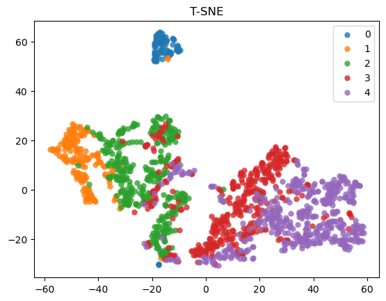
../_images/example_data_100_T-SNE.png — example_data_100_T-SNE.png

Confusion matrix (CM)

CM module evaluates classification accuracy by computing the confusion matrix with each row corresponding to the true class

Parameters	Optional	Descripton
-i, —input	filename path	dataframe path (CSV format)
—format	png, pdf	Picture format
—model_path	filename path	Model file path (joblib)
-n, —feature_number	int	feature number
-o, —output	directory	Output directory (default:Current directory)

CM example

# $Feature_scML automl -i example.csv -c svm -m fscore
$Feature_scML plot CM -i example_fscore_data.csv -n 100 --model_path example_100_svm.joblib

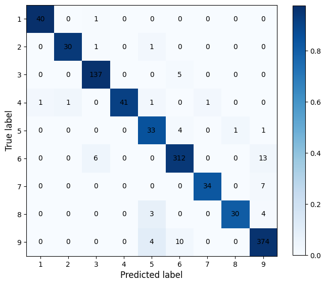
../_images/confusion_matrix_example_fscore_data_100.png — confusion_matrix_example_fscore_data_100.png